Optimising Portolio of ING PPS Funds

What is ING PPS (Private Portfolio Service) Funds?

Private Portfolio Service is a master trust administered by ING. It has been developed as both a series of unit trusts and a superannuation fund, representing a broad range of asset classes and fund managers.

Private Portfolio Service provides investors with the opportunity to diversify their portfolio, without the need to rebalance different investments across a number of fund managers and products.

Someone definitely has to do a quantitative research on these funds, right? What's the purpose? To find the best and optimised alocation of a portfolio of one's retirement plan or any investment plan.

Based on their daily/monthly historical prices, I calculated the daily/monthly log return of each PPS fund, Ln(P2) - Ln(P1) to show the continously compounded return.

I then calculated the mean and standard deviation of each fund and built the covariance matrix. Next, I calculated the portfolio mean and standard deviation.

Finally, using solver, the optimised allocation is found by assuming risk free rate 7%. Contact me to get the optimised allocation and the spreadsheet, if you're curious or just checking with your own calculation.

Please confirm if these annualised monthly means and standard deviations are close with your calculation for data ending 21 Jan 08.

PPS	mean	stdev
AggBal	7%	0.087
AsianEq	10%	0.159
AusEq	7%	0.126
Bal	5%	0.063
DivTrad	3%	0.041
EuroEq	6%	0.138
GlobOpp	-1%	0.176
InterEq	5%	0.131
InterFix	3%	0.029
Mortg	1%	0.018
NZEq	5%	0.098
NZFixed	0%	0.021
PlatInter	1%	0.101
Prop	6%	0.080

Some notes

Sorry, I didn't use CAPM return in this calculation. No market index benchmark therefore no beta and risk premium to consult. :-)

This is an optimisation of a portfolio of optimised funds as a managed fund is a portfolio which is optimised regularly by its fund managers.

Putting into practice, some clients don't believe in this simulation. This is because the simulation is based on the daily prices and they don't concern this kind of time horizon.

For getting the best point of view, in my opinion, it is best simulated from monthly prices, not daily prices.

Portfolio Optimisation (Shares & Funds)

It's quite a complex portfolio optimisation model which aims to find the optimised fund allocation in a portfolio of Australian and NZ managed funds with future return simulation using MonteCarlo method.

The historical prices are provided by Morningstar NZ and the copyright of this model is belong to Lyfords Ltd which I work with.

The optimisation is done by maximising the tangency portfolio (theta) so that it touches the edge of the efficient portfolio from the constant. There are also additional constraints such as particular conditions for any particular fund allocation. (eg. Thoroughbred Cash Fund = 5% and PPS Int Fixed Interest less than 10%)

If it applies into managed funds instead of shares, this may be an optimisation of a portfolio that may have been optimised (by fund managers) as a managed fund is in fact an optimised portfolio.

The process as follows:

1. Gathering data input: historical monthly fund prices. Calculate the historical monthly mean and stdevation of each asset.

2. Conduct a MonteCarlo simulation for monthly returns through 3 years horizon (36 months) using normal distributed random numbers using the historical montly mean and stdev at random probability.

3. Simulate the whole 3 years random movement. If simulated 10 times, so there are 36 monthly simulations times 10 three-yearly simulations (360). Record the projected mean and stdev.

4. Find the simulated portfolio return and risk using the projected mean and stdev.

5. Find the optimised portoflio expected return and risk.

6. Solve the optimised asset allocation using solver VBA. Apply additional constraints to reoptimise.

7. Calculate the value-at-risk.

Option to use mean or CAPM return is to choose whether CAPM is believed to be effective or not in this optimisation. If mean return is used then beta and risk premium don't matter.

Covariance matrix is also to be projected based on the simulation result.

Option to use historical or projected standard deviation is to choose whether portfolio risk is believed to be accumulated in the simulation result.

To run the Solver VBA.

1. Tools > Add-ins to have the Solver add-in first (in a file called Solver.xla)

2. Then create a reference to the 'Solver.xla' in Visual Basic Editor.
Go to Tools > Macro > Visual Basic Editor, choose Tools > References and check the box for Solver.

If it is missing, just click browse and manually find the "Solver.xla" file wherever it is located in your computer.

[Sorry, it's a premium model]

Live-updated Beta Calculation

Assume CAPM is applicable and works empirically without any doubt in the theory, we can then calculate a stock Beta dynamically over time as it represents the updated historical stock prices from the latest price. Hence, the stock Beta changes over time.

The process and the VBA coding are similar with the Live-updated Yield posted before.

This spreadsheet consists of 3 worksheets that dynamically calculates the beta of Astra stock returns (ASII.JK) against the Jakarta Composite index returns (^JKSE) as being updated over time by clicking the "Update" buttons. Thus, we can get the latest Beta of Astra stock.

The first worksheet is JKSE sheet that contains the recent updated market prices and the second one is ASII sheet for the recent updated stock prices. In these two sheets, there are two "Update" buttons that allow us to update the recent prices from web query and to record the recent prices into the Beta sheet (third worksheet).

The stock Beta is then calculated by simply finding the slope between the periodical stock (x axis) and market (y axis) returns.

[Sorry, it's a premium spreadsheet]

Comprehensive Financial Planning

An Excel model to judge your prosperity and set your financial goal and objectives.

[Sorry, it's a premium spreadsheet]

The comprehensive spreadsheet is premium, however, you can download this file: University and Pension Plans.

Uni & Pension Plan...

Hosted by eSnips

Value-at-Risk

Suppose you hold a portfolio like this.

Astra Int shares (ASII) with market value of IDR1,000,000,000.00
Indonesia Govt bonds (Indo-17) with market value of IDR1,000,000,000.00

Total market value of your portfolio is IDR2,000,000,000.00

You may wonder how much your portfolio value would be tomorrow in the worst-case scenario.

How do we get that value? Such value is known as Value-at-Risk (VaR).

The procedure:
1. Collect historical daily data for Astra share prices and calculate the daily return.
2. Collect historical daily date for Indonesia govt bonds yields, generate index and calculate the daily return.
3. Generate covariance matrix for share return and bond return.
4. Calculate portfolio variance and standard deviation. In Excel, it can be done using MMULT(MMULT(TRANSPOSE(value),covariancematrix),value)
5. Calculate VaR at 99% confidence level as 2.326 multiply by standard deviation.
6. Tomorrow's worst value = Today's value - VaR

From the example, I found tomorrow's worst case value is IDR1,937,346,708.11

[Sorry, it's a premium spreadsheet]

Bond Price, Duration and Convexity

In Feb 06 I submitted some short of article in Wikipedia about closed form formulas for bond duration and convexity. Below is the clone and hopefully it can be useful for those who may use the formulas for bond analysis modelling in Excel spreadsheets.

As far as I know, these have never been published on the web like this as I experienced some problem in finding them when doing some bond pricing project.

Closed-form formula:
A single arithmetic formula obtained to simplify an infinite sum in a general formula. The general formula of bond duration and bond convexity cannot be said closed-form as there is an infinite sum over the different time periods. Using a closed-form formula, a bond’s duration or convexity can be calculated at any point in its life time.

Bond duration closed-form formula (Richard Klotz):


C = coupon payment per period (half-year)
P = present value (price)
i = discount rate per period (half-year)
a = fraction of a period remaining until next coupon payment
m = number of coupon dates until maturity

Bond convexity closed-form formula (Blake and Orszag):


D = coupon payment per period
P = present value (price)
B = face value
i = discount rate per period (half-year)
a = fraction of a period remaining until next coupon payment
m = number of coupon dates until maturity

[Sorry, it's a premium spreadsheet]

Live-updated Yield

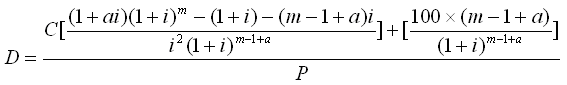
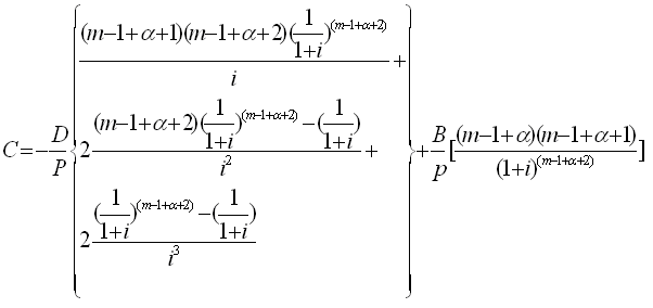
The purpose of this model is to provide a live-updated spreadsheet by automatically capturing the current data provided by a website via Web Query and then automatically recording the data into a master data sheet through a Bootstrapping method.

So, it's just two clicks away on our spreadsheet to update a time series graph to the current rate, automatically. It's similar when we are running a live-update for our antivirus software.



The Worksheet

[Sorry, it's a premium spreadsheet]


The Sheets

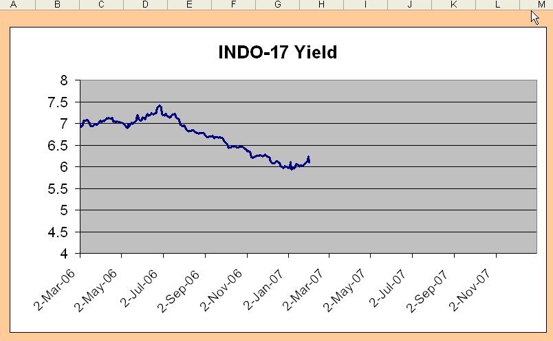
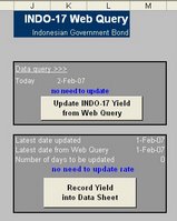
There are three sheets: INDO17, Data and Graph. "INDO17" is a sheet where the web query should go and where the two updating clicks are available. "Data" is a sheet where the bootstrapping process is running. "Graph" is only for visualisation.


Cell Naming

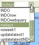
Cell naming is an important method as explained before in the previous post. There are several cells to be named in this worksheet and used for visual basic coding: INDO, INDOrow, INDOwebquery, nodays and updatelatestINDO.

To find which range is referred by a cell name, just go to the box on the top left, scroll the box and click the name. A range or cell will be shown.

• INDO: a range as the destination for the updated rate from 2-Mar-06 to 31-Dec-10 in "Data" sheet (B5:B1263).
• INDOrow: a cell showing a number of rows from 2-Mar-06 to the latest date has been updated in "Data" sheet (D3).
• INDOwebquery: a range as the source of data captured via web query in "INDO17" sheet (A2:D21).
• nodays: a cell showing a number of days need to be updated since the last updated date in "INDO17" sheet (M14).
• updatelatestINDO: a cell showing the next date needs to be updated in "Data" sheet (G4).

Visual Basic Coding

Web Query Update
This code is for the first button "Update INDO-17 Yield from Web Query". The webpage source used for web query is the INDO-17 yield data provided in the Central Bank of Indonesia website.

The code:

Sub dailyINDO()

Application.OnTime Now + TimeValue("12:00:00"), "updateINDO"

End Sub

Sub updateINDO()

Sheets("INDO17").Activate
Range("a1").Select
Selection.QueryTable.Refresh BackgroundQuery:=True
dailyINDO

End Sub

Recording Data through Bootstrapping
This code is for the second button "Record Yield into Data Sheet". The code is quite complicated. However, if we can follow the logic and as referring to the range names, this is a piece of cake for us.

The code:

Sub recordINDO()

For j = 1 To Range("nodays")
For i = 1 To Range("nodays")

If Sheets("Data").Range("updatelatestINDO") = Range("INDOwebquery").Cells(i, 1) Then
Range("INDOwebquery").Cells(i, 4).Copy

r = Sheets("Data").Range("INDOrow") + 1

Sheets("Data").Range("INDO").Cells(r).PasteSpecial Paste:=xlPasteValues
Calculate
End If

Next i
Next j

Sheets("Data").Select

End Sub

The meaning of the above code is:

For the loops as many as the number of days needs to be updated, Excel will copy each yield in the web query sheet and paste into the data sheet on each corresponding date. Where the corresponding date is found by referring the number of rows from the first date to the latest updated date plus 1 day after.

Piece of cake, aye?

Option for updating screen
You may insert this code to disable the visualisation of screen updating. Meaning, you can't see the price line moving forward as time moves.

Application.ScreenUpdating = False


The "INDOrow"

It seems the key problem here is to find the number of "INDOrow", a cell showing a number of rows from 2-Mar-06 to the latest date has been updated in "Data" sheet (D3).

The way is using a MATCH function to calculate the number of rows from 2-Mar-06 to the latest date as this formulae:
=MATCH("latest date",C5:C498,0)

Where the "latest date" is found by tagging a note in the column C as the latest date using IF formulae: =IF(AND(the next yield=0, the current yield >0),"latest date","").


The "updatelatestINDO"

This is a cell showing the next date needs to be updated in "Data" sheet (G4) that can be found easily using an INDEX function:

=INDEX($A$5:$A$498,INDOrow+1)


Recommendation and Notes

The title is for updating government bond yield, but the application can be also for updating other time series data such as foreign exchange rates or share prices.

I also open for any suggestions particularly for any more simple VBA codes.

Please let 2 days lag from Bank Indonesia website for current rate. It doesn't mean they are lazy to update, they just have a lot of other things to do.

Dynamic Company Valuation

Since the key parameters in valuation model are mostly influenced by market behaviour, then it is important to update some relevant market data in regular basis to see how they affect the analysis. The relevant market data may include risk-free rate, stock price and market index that are able to indicate changes in value.

This model introduces manipulation of data by automatically changing some market data via the tool of external data import in Excel and some VBA simple codes for refreshing the Web Query. The main goal is to adjust calculation in Beta and WACC in the framework of company valuation and also for Option and Bond analysis.

In projecting financial statement, the historical data of the last two year operation is used to find the assumptions in the form of financial ratios that are normally corresponded to Sales. Then, the average of the last two year ratios can be used as the basic assumptions. Sales Growth ratio can be used as a look-up parameter in sensitivity analysis.

Sensitivity models are used by utilising two important tools in Excel, i.e., Data Tables and Graphs. Both tools are set to show visual changes in value after altering the growth ratio to some levels. This model also introduces sensitivity analysis of changes in financial ratios for the goal of predicting the possibility of bankruptcy. Traditional financial ratio techniques used are for Altman Bankruptcy model and Chesser Loan Surveillance model to be visually compared with the equity value and stock price resulted from the Free Cash Flow valuation.

The key analysis in this model is the Free Cash Flow valuation that has been as the important technique explained in the course and from the text. The method follows the that has been explained in the class using the No-Negative Cash and Debt as the Plugs. Some modification is tried to be applied by using Bonds as the plug, where the Bank Loans is calculated based on the bank loans to bonds ratio. The sum of both is the Long-term Debt.

Using bonds as the plug, the plan is to set of a Bond Portfolio for covering future financing in the projection. Then, the analysis refers to Net Present Value and Portfolio Duration that may anticipate in the future. As a bond issuer, the company should expect the lower value and duration.

[Sorry, it's a premium spreadsheet]

Bond Portfolio Analysis

Using the closed-form bond formula posted before, this bunch of spreadsheet is produced to value a bond at any point in its life time and do some analyses, as follows:

• Portfolio valuation, duration and convexity
• Derivatives valuation: FRA, Swap, Futures
• Risk governance: Value-at-Risk, Stress Testing and Scenario Analysis
• Hedging effectiveness
• Liquidity analysis

Remark: this portfolio is a liability/debt portfolio, NOT an asset/investment portfolio.

[Sorry, it's a premium spreadsheet]